Tutorial: build a map

This tutorial describes the steps for building metric maps using MOLA.

---

---

1. Prepare the input data

• Think what sensors do you want to use:

  • At least, one 2D or 3D LiDAR. It is possible to have multiple LiDARs.

  • Optional: Encoder-based odometry, for wheeled robots.

  • Optional: Low-cost GNSS (GPS) receiver, for georeferencing the final metric maps. You can use mrpt_sensor_gnss_nmea for standard GNSS USB devices providing NMEA messages.

• Decide whether SLAM will run online (live) or offline (in postprocessing).

• If running offline (recommended): Grab the data using ros2 bag record if you use ROS 2. Alternative options include using MOLA-based dataset sources.

• If using ROS 2…

  • …and you only have one LiDAR as the unique sensor, then setting up ROS tf frames is not mandatory, if you are happy with tracking the sensor pose (vs the vehicle pose).

  • …and you have wheels odometry or additional sensors on the robot, then having correct /tf messages published is important to let the mapping algorithm know what is the relative pose of the sensor within the vehicle.

• Even if having only one single LiDAR, correctly defining the sensor pose on the vehicle is important for correctly tracking the vehicle pose instead of the sensor pose. This can be done by either…

  • correctly setting up /tf, or

  • using the MOLA-LO applications flag to manually set the sensor pose on the vehicle without /tf.

2. Run MOLA-LO

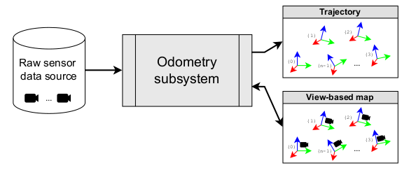
The output of running LiDAR odometry on your dataset is a an estimated trajectory and a simple-map (here is the main stuff to build maps from):

Role of an “odometry” module (Figure adapted from [BC24]).

To process an offline dataset, use any of the available options in MOLA-LO applications:

• mola-lo-gui-rosbag2 for a version with GUI, or

• mola-lidar-odometry-cli for a terminal (CLI) version.

To launch SLAM live on a robot, read how to launch the MOLA-LO ROS 2 node.

In any case, make sure to enable the option of generating and saving the output simple-map and take note of where is the generated file. This can be done via environment variables before launching MOLA-LO, or from the UI controls in the mola_lidar_odometry subwindow.

Use these commands to get going

For quickly getting MOLA-LO running, you can start using these commands, although it is recommended to later go through the documentation linked above to learn about all the possibilities:

From a rosbag2 (GUI)

MOLA_LIDAR_TOPIC=/ouster/points \
MOLA_GENERATE_SIMPLEMAP=true \
MOLA_SIMPLEMAP_OUTPUT=myMap.simplemap \
MOLA_SIMPLEMAP_GENERATE_LAZY_LOAD=true \
  mola-lo-gui-rosbag2 /path/to/your/dataset.mcap

Note

Remember changing MOLA_LIDAR_TOPIC to your actual raw (unfiltered) LiDAR topic (sensor_msgs/PointCloud2).

From a rosbag2 (CLI)

MOLA_SIMPLEMAP_GENERATE_LAZY_LOAD=true \
mola-lidar-odometry-cli \
  -c $(ros2 pkg prefix mola_lidar_odometry)/share/mola_lidar_odometry/pipelines/lidar3d-default.yaml \
  --input-rosbag2 /path/to/your/dataset.mcap \
  --lidar-sensor-label /ouster/points \
  --output-tum-path trajectory.tum \
  --output-simplemap myMap.simplemap

Note

Remember changing --lidar-sensor-label /ouster/points to your actual raw (unfiltered) LiDAR topic (sensor_msgs/PointCloud2).

From a rosbag2 (CLI) (Large datasets)

For maps large enough such as the final .simplemap does not fit in RAM, you can enable lazy-load simplemap generation in the CLI with:

MOLA_GENERATE_SIMPLEMAP=true \
MOLA_SIMPLEMAP_GENERATE_LAZY_LOAD=true \
MOLA_SIMPLEMAP_OUTPUT=myMap.simplemap \
mola-lidar-odometry-cli \
  -c $(ros2 pkg prefix mola_lidar_odometry)/share/mola_lidar_odometry/pipelines/lidar3d-default.yaml \
  --input-rosbag2 /path/to/your/dataset.mcap \
  --lidar-sensor-label /ouster/points \
  --output-tum-path trajectory.tum

Note

Remember changing --lidar-sensor-label /ouster/points to your actual raw (unfiltered) LiDAR topic (sensor_msgs/PointCloud2).

Building 2D maps

Until mola_2d_mapper is released, you can also use the generic LiDAR odometry module to build 2D maps from range finder (2D scanners).

Just set the PIPELINE_YAML environment variable pointing to the 2D mapping pipeline (lidar2d.yaml) shipped with the mola_lidar_odometry package:

MOLA_LIDAR_TOPIC=/scan1 \
PIPELINE_YAML=$(ros2 pkg prefix mola_lidar_odometry)/share/mola_lidar_odometry/pipelines/lidar2d.yaml \
MOLA_GENERATE_SIMPLEMAP=true \
MOLA_SIMPLEMAP_OUTPUT=myMap.simplemap \
  mola-lo-gui-rosbag2 /path/to/your/dataset.mcap

Remember to change /scan1 to your actual topic name of type sensor_msgs/LaserScan.

Hint

To help you getting familiar with the whole process, feel free of downloading any of these example simple-maps so you can use follow the rest of the tutorial before building your own maps:

• mvsim-warehouse01.simplemap : A map of a (simulated) warehouse, built from a wheeled robot with a 3D LiDAR.

3. Inspect the resulting simple-map

To verify that the generated simple-map is correct, you can use sm-cli.

Examples

These examples assume you have downloaded mvsim-warehouse01.simplemap, but can be also applied, of course, to your own maps:

Basic information

sm-cli info mvsim-warehouse01.simplemap

Output:

Loading: 'mvsim-warehouse01.simplemap' of 46.77 MB...

size_bytes:           46771378
keyframe_count:       77
has_twist:            true
kf_bounding_box_min:  [-13.275376 -11.909915 -0.003725]
kf_bounding_box_max:  [19.122171 11.847500 0.364639]
kf_bounding_box_span: [32.397546 23.757415 0.368364]
timestamp_first_utc:  2024/01/03,11:25:30.875170
timestamp_last_utc:   2024/01/03,11:31:19.875170
timestamp_span:       05min 49.000s
observations:
  - label: 'lidar1'
    class: 'mrpt::obs::CObservationPointCloud'
    count: 77
  - label: 'metadata'
    class: 'mrpt::obs::CObservationComment'
    count: 77

Plot keyframes

sm-cli export-keyframes mvsim-warehouse01.simplemap --output kfs.tum
evo_traj tum  kfs.tum -p --plot_mode=xy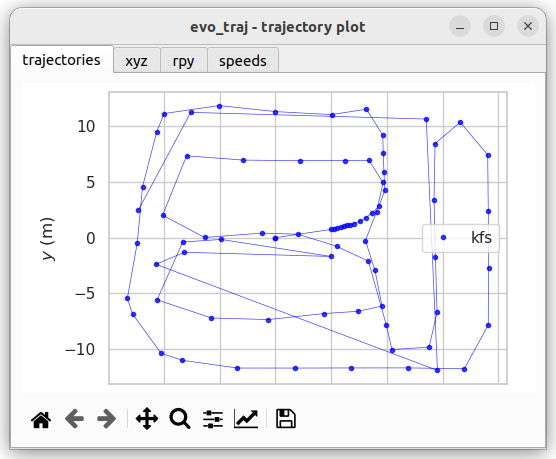

See stored LiDAR scans

sm-cli export-rawlog mvsim-warehouse01.simplemap --output warehouse.rawlog
RawLogViewer warehouse.rawlog

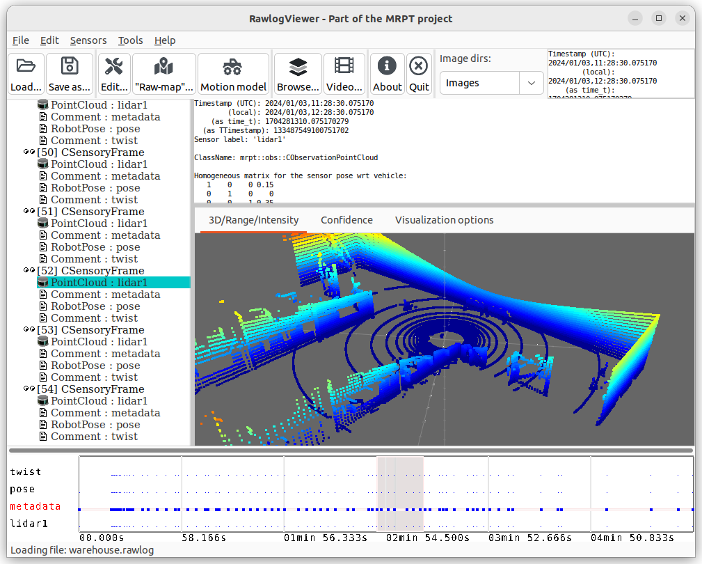
4. Build metric maps and visualize them

Generating metric maps from a simple-maps is done with mp2p_icp filtering pipelines. It can be done directly from C++ if so desired, or easily from the command line with sm2mm.

Afterwards, visualizing metric map files (*.mm) can be done with mm-viewer.

Examples

These examples assume you have downloaded mvsim-warehouse01.simplemap, but can be also applied, of course, to your own maps:

Build an aggregated 3D point cloud

Download the example pipeline sm2mm_pointcloud_voxelize_no_deskew.yaml and then run:

# Build metric map (mm) from simplemap (sm):
sm2mm \
 -i mvsim-warehouse01.simplemap \
 -o mvsim-warehouse01.mm \
 -p sm2mm_pointcloud_voxelize_no_deskew.yaml

# View mm:
mm-viewer mvsim-warehouse01.mm

Build a voxel map + 2D grid map

Download the example pipeline sm2mm_bonxai_voxelmap_gridmap_no_deskew.yaml and then run:

# Build metric map (mm) from simplemap (sm):
sm2mm \
  -i mvsim-warehouse01.simplemap \
  -o mvsim-warehouse01.mm \
  -p sm2mm_bonxai_voxelmap_gridmap_no_deskew.yaml

# View mm:
mm-viewer mvsim-warehouse01.mm

5. Publish the map to ROS 2

Publishing metric maps (*.mm files) as ROS topics for other nodes to use them is the purpose of the mrpt_map_server package. Please, read carefully its documentation to learn about all available features and parameters.

Map publish example

This example assumes you built mvsim-warehouse01.mm following instructions above.

To publish maps you need to install mrpt_map_server. The easiest way is:

# Make sure mrpt_map_server is installed:
sudo apt install ros-${ROS_DISTRO}-mrpt-map-server

In a terminal, run:

# Publish all map layers as ROS 2 topics:
ros2 launch mrpt_map_server mrpt_map_server.launch.py \
  mm_file:=$(pwd)/mvsim-warehouse01.mm

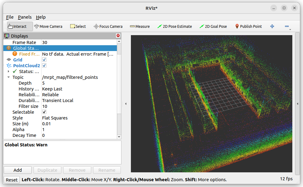
Next, open rviz2 in another terminal, and:

• Add a new display object of type PointCloud2 linked to the topic /mrpt_map/filtered_points.

• Make sure of changing its Durability to “transient local”.

6. See the inner workings of ICP

If you are interested in learning about the internal workings of each ICP optimization, or if there is something wrong at some particular timestamp and want to debug it, you can enable the generation of ICP log files and then visualize them with the GUI app icp-log-viewer.

Debug ICP

First, re-run MOLA LO enabling the generation of ICP log files (see all the available options):

# Generate ICP log files:
MP2P_ICP_GENERATE_DEBUG_FILES=1 \
MP2P_ICP_LOG_FILES_DECIMATION=1 \
mola-lo-gui-rosbag  [...]  # the rest remains the same

You should now have a directory icp-logs with as many files as times ICP invocations. Then, visualize the logs in the GUI with:

# Open the logs:
icp-log-viewer -d icp-logs/ -l libmola_metric_maps.so

7. What’s next?

Once you have a map, here are some next steps:

• loop closure (Write me!)

• Georeferencing.

• Use for localization.